



In this ten-minute beginner lesson, learners build a one-page oil market map using entirely fictional WTI-style and Brent-style crude oil benchmarks. They learn what an oil barrel measures, why benchmark prices differ, how crude quality and transportation affect pricing, and how to interpret inventory changes relative to expectations. A simulated WTI-style price of $70.00 and Brent-style price of $74.00 produce a $4.00 benchmark spread, while an invented transport and quality decomposition explains its components. Learners compare light sweet and heavy sour crude, calculate a hypothetical quality discount, and analyze a fictional weekly inventory report showing 420.0 million barrels of stocks against a 440.0 million five-year average. They identify a 2.5-million-barrel weekly draw, a 3.5-million-barrel bearish inventory-change surprise relative to the expected build, and 21 days of supply using fictional daily demand. Storage utilization, refinery throughput, contract multipliers, notional exposure, and price sensitivity complete the comparison. The outcome is the ability to distinguish WTI and Brent pricing concepts, interpret inventory surprises without predicting prices, and recognize why contract specifications matter before any simulated oil trade. All market prices, inventory figures, refinery data, assumptions, and contracts are fictional; no investment advice, real trading, or price predictions are provided.
What an Oil Barrel and a Benchmark Actually Mean
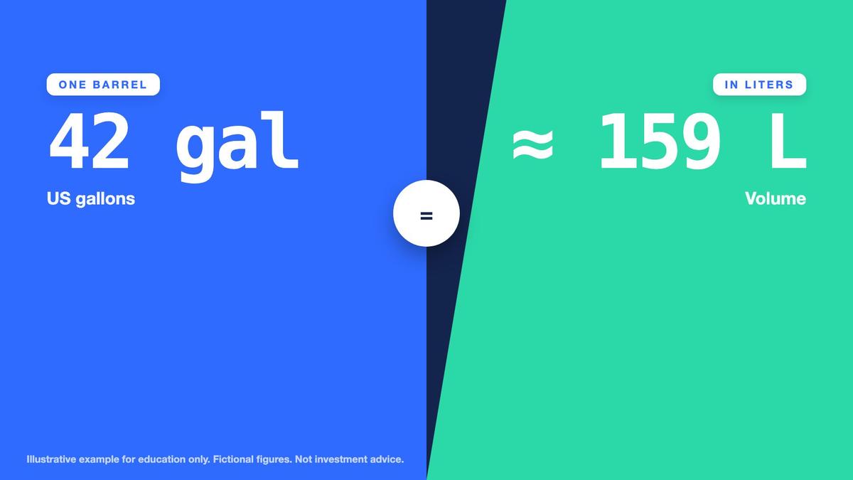
Crude oil is commonly quoted in dollars per barrel, but learners should first understand what the unit measures. A standard oil barrel represents 42 US gallons, approximately 159 liters. It measures volume, not the market value of a contract or the amount of cash required to obtain price exposure. A quotation of $70 per barrel describes the price assigned to one barrel under a specified market convention. To calculate a larger economic exposure, multiply the barrel price by the number of barrels represented. Before treating a quotation as tradable, identify the grade, delivery basis, instrument type, quotation timestamp and contract multiplier.


WTI stands for West Texas Intermediate and is closely associated with inland North American crude oil production, infrastructure and pricing. Brent is associated with crude oil from the North Sea region and functions as a major reference for seaborne international oil pricing. These descriptions identify broad benchmark roles rather than identical trading or delivery terms across every product carrying those names. A physical crude purchase, a futures contract, a listed product and a broker derivative may all reference a benchmark without providing the same rights or responsibilities. The precise legal structure, settlement mechanism and underlying quality definitions must be checked in the relevant instrument documentation.

Key points
- A barrel is 42 US gallons (about 159 liters): a unit of volume, not ownership or value.
- A benchmark is a widely referenced price for a defined crude market; WTI is tied to inland North America, Brent to seaborne pricing.
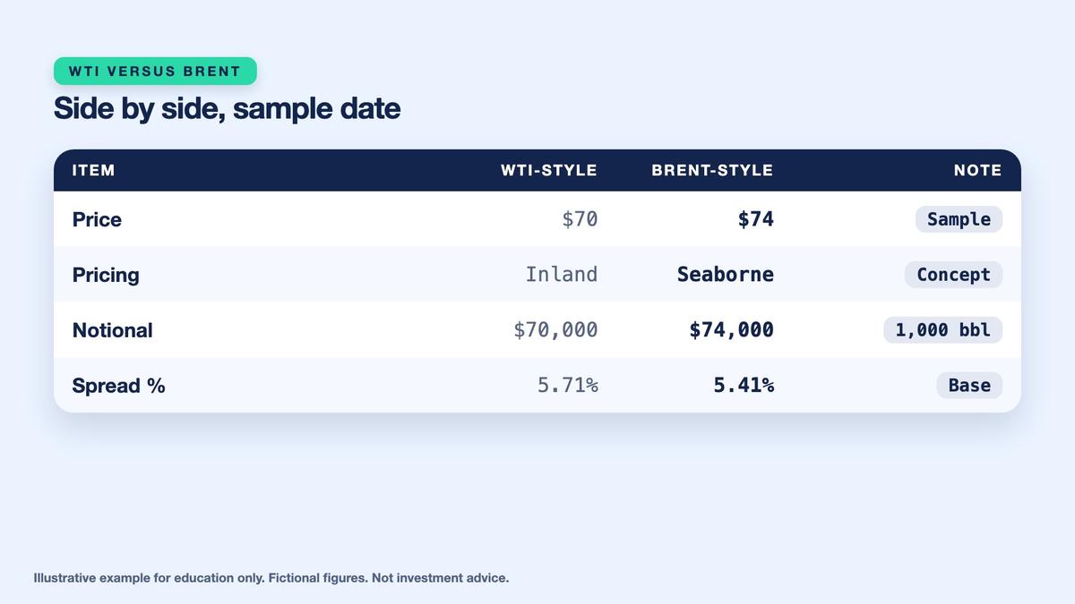
- Fictional sample date: WTI-style $70.00 and Brent-style $74.00 per barrel. Always verify the real contract terms.
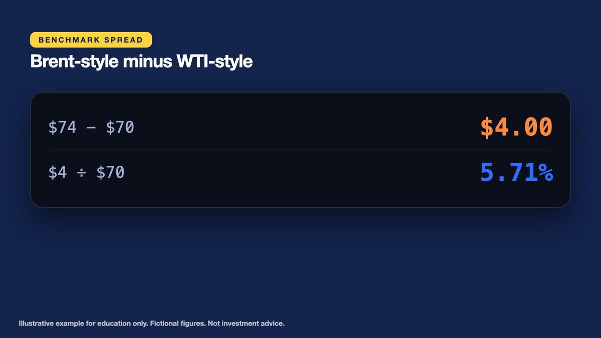
Our single fictional worked example starts with a WTI-style quotation of $70.00 per barrel and a Brent-style quotation of $74.00. The prices are invented for a sample date and are not actual market quotes or forecasts. The simple benchmark difference is $74.00 minus $70.00, equal to $4.00 per barrel. Relative to the $70 WTI-style price, the difference is 4 divided by 70 times 100, approximately 5.71%. Relative to the $74 Brent-style price, it is approximately 5.41%. These percentages differ because their denominators differ, not because the underlying four-dollar price gap changes.
Why WTI and Brent Can Have Different Prices
A benchmark price reflects more than the chemical composition of crude oil. Geography, transportation links, delivery points, export access, refinery demand and the market's willingness to hold inventories can all influence relative prices. An inland barrel may face different transport options than a barrel available at a seaborne terminal. Differences in freight costs, pipeline capacity, shipping schedules and regional demand can therefore contribute to a spread between benchmark quotations. None of these relationships has a fixed universal value. Their importance can change with weather, infrastructure disruptions, international trade and shifting crude flows.
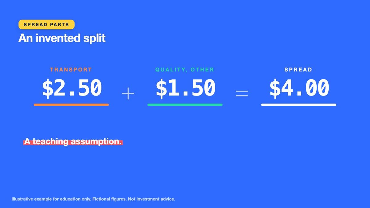
For our fictional sample, decompose the $4.00 WTI-style to Brent-style spread into $2.50 per barrel associated with transportation and shipping and $1.50 associated with crude quality and other market factors. The two components add to exactly $4.00. This is an invented explanatory allocation, not a documented empirical decomposition. Across the fictional 1,000-barrel contract used later in the lesson, the $2.50 transport portion corresponds to $2,500, while the $1.50 quality-and-other portion corresponds to $1,500. Together they represent $4,000 of reference value difference for equal quantities at the two prices.
Key points
- Spread = $74.00 - $70.00 = $4.00 per barrel: 4 / 70 = 5.71% of the WTI-style price (4 / 74 = 5.41% of Brent-style).
- Invented split: $2.50 transport and shipping + $1.50 quality and other = $4.00.
- A spread is not automatic profit; costs, delivery terms and timing matter.
The benchmark spread is not automatically an arbitrage profit. Buying one crude grade and selling another can require transportation, storage, financing, product substitution, delivery timing, contractual rights and execution at available market prices. Futures and broker contracts may also reference different months, settlement procedures or instruments. Consequently, a visible $4 difference does not demonstrate that the learner could capture $4 per barrel without risk. The practical habit is to label both benchmark quotations, their units, their sample date and their underlying delivery conventions before interpreting a price comparison. This follows the exposure-mapping approach introduced in the earlier gold lesson.
Crude Quality: API Gravity, Sulfur and Refinery Preference
Crude oil grades can differ in density, sulfur content and the types of products that refineries can economically produce from them. API gravity is a petroleum industry measure related to relative density; higher API gravity generally indicates lighter crude. Light and heavy are comparative descriptions rather than a guarantee of a specific selling price. Sweet and sour commonly distinguish lower-sulfur from higher-sulfur crude, although precise classifications can vary. Refineries with different equipment and configurations may prefer different feedstocks. A more complex refinery can sometimes process heavier or higher-sulfur barrels that another facility finds less desirable.
Our fictional Sample Light Sweet crude has 40 degrees API gravity and sulfur content of 0.4%. Sample Heavy Sour crude has 30 degrees API gravity and 2.0% sulfur. These are invented laboratory descriptions for the example. Assume the light sweet grade is priced at the $70.00 per-barrel reference, while the heavy sour grade receives a fictional $6.00 discount. The heavy sour price is therefore $64.00 per barrel. Calculating 6 divided by 70 times 100 gives approximately 8.57%. This discount is an assumption about the example, not a universal statement that heavier or more sulfurous crude always trades at a fixed reduction.

Key points
- Light sweet: 40 degrees API, 0.4% sulfur. Heavy sour: 30 degrees API, 2.0% sulfur.
- Invented discount: $6 below $70, so $64, or 6 / 70 = 8.57%.
- Quality changes price through refinery fit and processing costs, but this relationship is only a teaching assumption.
Quality affects price through processing costs, product yields, refinery capabilities and the availability of different crude grades. Sulfur removal and upgrading equipment can be expensive to operate, but refinery economics also depend on the selling prices of gasoline, diesel and other products. A quality differential can narrow or widen even if the headline benchmark prices remain stable. The learner should therefore record the specific grade attributes, not simply label one crude better than another. In the oil market map, include the two API gravity readings, the sulfur percentages, the six-dollar fictional discount and the fact that actual values depend on refinery demand and local market conditions.
Read Inventory Reports: Actual Change Versus Expected Change
Crude oil inventories represent stocks held in storage at particular locations and within particular reporting definitions. Weekly inventory reports can help analysts assess whether oil is accumulating or being drawn down, but their significance depends on what the market expected. A build means reported stocks increased over the period. A draw means reported stocks decreased. Neither word alone determines a future price movement. Refinery operations, imports, exports, domestic production, transportation movements and reporting conventions can all influence the weekly change. A market price may already reflect an anticipated draw or build before the report appears.
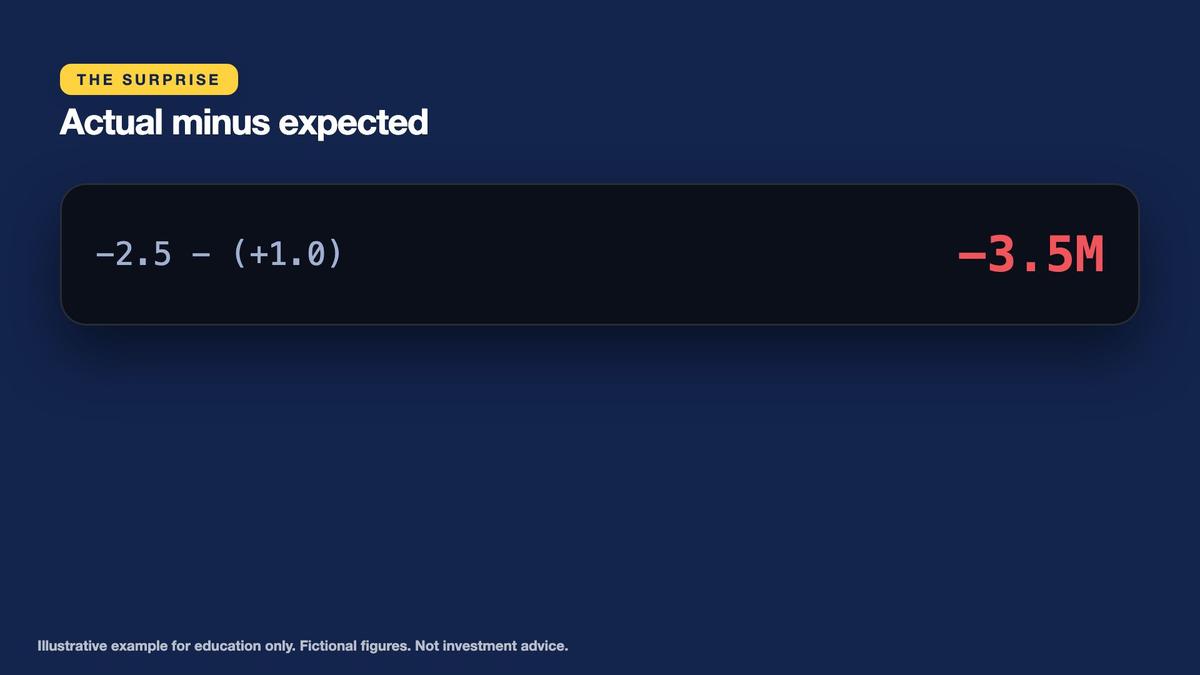
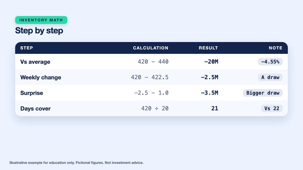
Open the fictional weekly report. Current crude stocks are 420.0 million barrels, compared with a previous-week figure of 422.5 million. Subtract previous stocks from current stocks to obtain 420.0 minus 422.5, or negative 2.5 million barrels. The actual change is therefore a 2.5-million-barrel draw. Before the report, the invented market consensus expected a positive 1.0-million-barrel build. The surprise is actual change minus expected change: negative 2.5 minus positive 1.0 equals negative 3.5 million barrels. The market received a reported draw instead of the expected build, making the result substantially different from the prior assumption.
Key points
- Stocks 420.0M barrels; previous week 422.5M; actual change 420.0 - 422.5 = -2.5M (a draw).
- Expected +1.0M, so the surprise = -2.5 - (+1.0) = -3.5M.
- A larger draw than expected suggests tighter supply; a larger build suggests looser. A signal of direction, not a forecast.
Under the classroom reading rule, a larger-than-expected draw suggests supply may be tighter than market participants anticipated. Conversely, a larger-than-expected build can suggest looser conditions. These are interpretive signals, not forecasts or guarantees. Oil prices can respond to producer decisions, economic announcements, demand revisions, geopolitics, currency developments and existing market positions at the same time. A negative inventory surprise does not require a positive price return, and different parts of the futures market may react differently. The learner should journal the actual stocks, previous stocks, expected change, actual change, calculated surprise and a note that directional interpretation remains uncertain.
Compare Stocks With History and Calculate Days of Supply
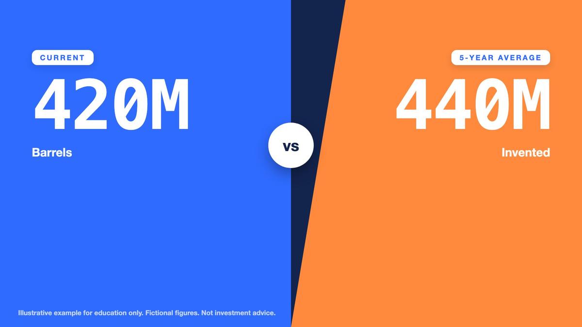
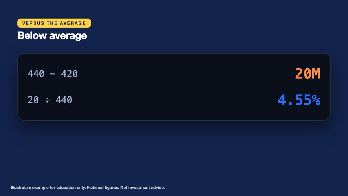
The fictional weekly report also provides an invented five-year average inventory of 440.0 million barrels. Current stocks of 420.0 million are therefore 20.0 million barrels below that reference. Dividing the 20.0-million shortfall by the 440.0-million average and multiplying by 100 yields approximately 4.545%, displayed as 4.55% below average. This comparison describes the relationship between one current fictional stock observation and a historical reference. A historical average is not automatically a normal or desirable stock level, because refinery demand, transportation systems, production patterns and other market conditions can change over time.
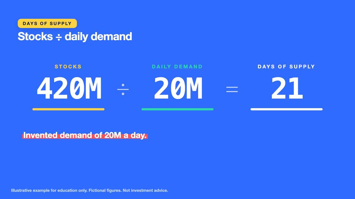
Days of supply translates a stock quantity into an illustrative consumption horizon. Assume fictional crude demand equals 20.0 million barrels per day. Divide current stocks of 420.0 million barrels by that daily demand to obtain 21.0 days. Apply the same denominator to the invented five-year average of 440.0 million barrels to obtain 22.0 days. The current figure is therefore one day lower than the historical reference under constant demand. This calculation helps compare inventory relative to consumption rather than relying only on total barrels. It is especially useful when comparing different periods or hypothetical economic conditions.
Key points
- Five-year average 440.0M: stocks are 20.0M below, 20 / 440 = 4.55%.
- Days of supply with invented demand of 20.0M a day: 420 / 20 = 21.0 days, against 440 / 20 = 22.0.
- Days of supply is a simplified ratio, not a countdown to empty tanks.
Days of supply is not a literal countdown until oil disappears. A petroleum market continues producing, importing, exporting and processing crude while storage levels fluctuate. Some inventory may be unavailable for normal commercial use, and reported coverage depends on what stocks and demand categories the calculation includes. The learner must write the numerator and denominator explicitly: 420.0 million barrels of fictional crude stocks divided by 20.0 million barrels of assumed daily demand. Do not substitute refinery throughput for overall demand without recognizing that the variables describe different activities. The oil map should retain both the 21-day current calculation and the 22-day historical comparison.
Why Storage Capacity and Refinery Runs Matter
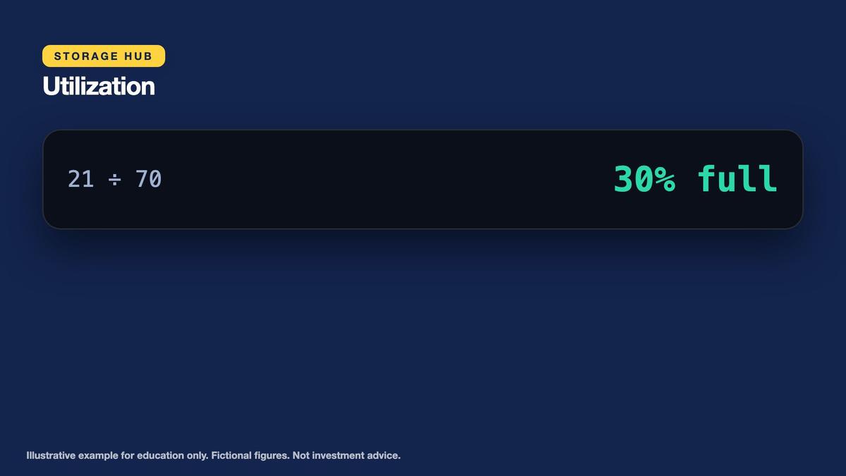
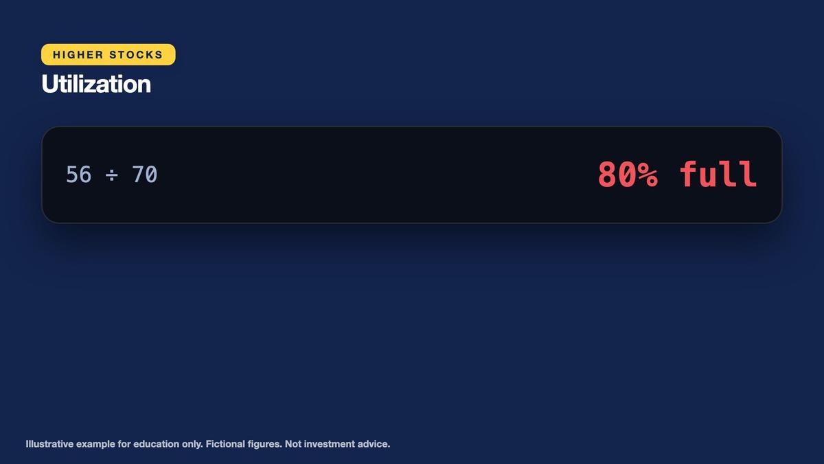
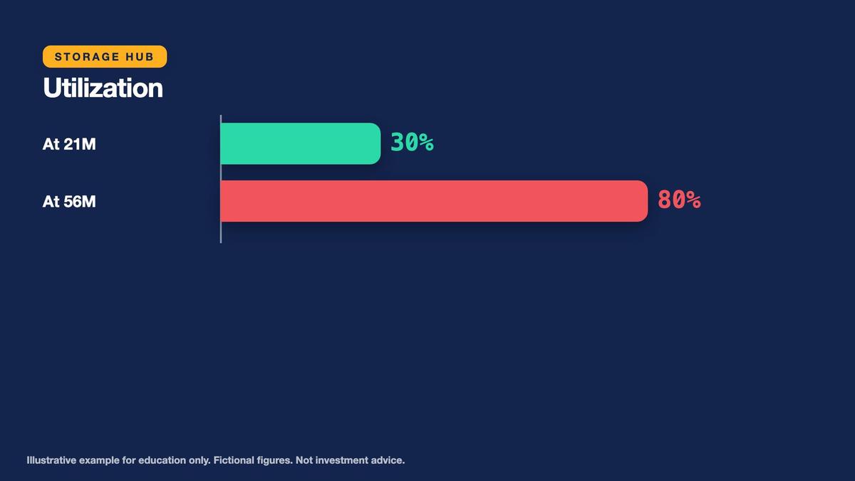
Oil storage is physical infrastructure with finite capacity, location constraints and operating requirements. Our fictional storage hub has nominal capacity for 70.0 million barrels and currently holds 21.0 million. Dividing stocks by capacity gives 21 divided by 70, or 30% utilization. Under a separate hypothetical condition, hub inventories rise to 56.0 million barrels. Utilization then becomes 56 divided by 70, or 80%. Nominal unused space falls from 49.0 million barrels at the first level to 14.0 million at the second. Operationally available capacity can differ from nameplate capacity because tank availability, maintenance, product segregation and logistics create practical restrictions.
Storage fullness can influence the economics of nearby physical delivery. If a hub approaches its usable capacity and incoming barrels cannot easily move elsewhere, buyers may demand larger discounts to accept immediate deliveries. Conversely, scarce inventories or difficult replacement supply can support the value of readily available crude. These relationships are conditional and depend on the precise delivery point, grade, timing and alternative transport routes. The fictional move from 30% to 80% utilization demonstrates why inventory location matters independently of a national aggregate. It does not establish a universal price threshold at 80%, nor does it predict a particular benchmark spread.
Key points
- Hub capacity 70.0M barrels: at 21.0M it is 21 / 70 = 30% full; at 56.0M it is 56 / 70 = 80% full.
- A nearly full hub can pressure prices for nearby delivery.
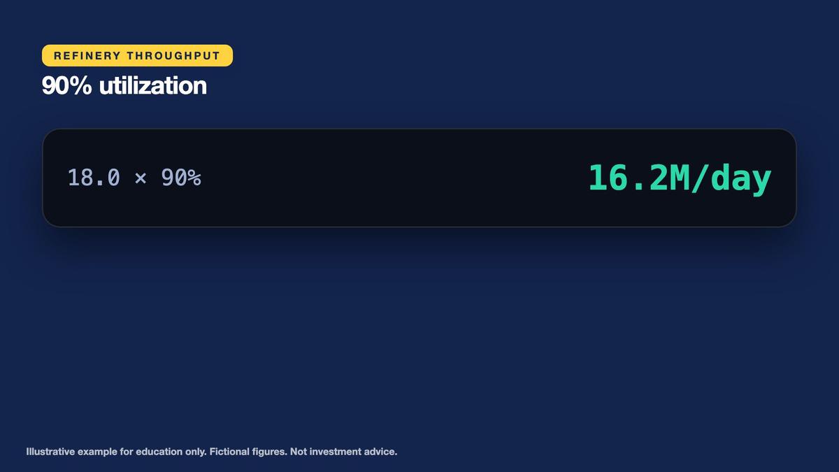
- Refining: 18.0M barrels a day at 90% = 16.2M; at 95% = 17.1M of crude processed.
Refineries consume crude oil as feedstock and therefore influence crude demand. Assume our fictional refining system has capacity for 18.0 million barrels per day. At 90% utilization, crude throughput equals 18.0 multiplied by 0.90, or 16.2 million barrels per day. At 95% utilization, throughput equals 17.1 million barrels per day, an increase of 0.9 million. Higher refinery runs can increase crude intake if feedstock supply, product demand and other operating conditions permit. Refinery throughput is not identical to final consumer demand or crude inventories. The learner should record refinery capacity, utilization and resulting throughput as separate fields in the oil map.
Convert Oil Prices Into Contract Exposure and Risk
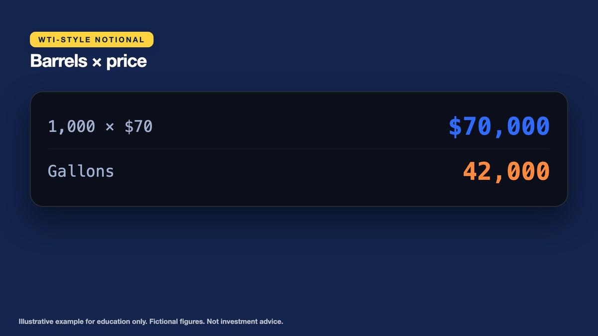
To connect physical market fundamentals with financial exposure, introduce a fictional oil contract representing 1,000 barrels. The contract size is a case assumption, not a universal specification for every real instrument. At 42 US gallons per barrel, the contract represents 42,000 US gallons of oil volume. A $1 price movement per barrel creates a $1,000 change in gross contract value because 1,000 barrels are multiplied by the one-dollar movement. The price sensitivity applies symmetrically: a favorable one-dollar change produces $1,000 gross gain, while an unfavorable one-dollar change produces $1,000 gross loss, before commissions, spreads, slippage or financing.

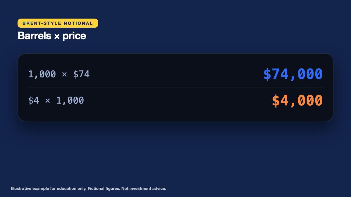
At the invented $70.00 WTI-style reference, 1,000 barrels represent $70,000 notional. At the invented $74.00 Brent-style reference, the same barrel quantity represents $74,000 notional. Their $4.00-per-barrel benchmark gap corresponds to $4,000 across 1,000 barrels. The invented decomposition assigns $2,500 of that difference to transportation and shipping and $1,500 to quality and other factors. This scaling is arithmetic rather than a trading strategy. Two benchmark contracts can differ in expiry, currency, settlement, delivery quality and execution liquidity, so comparing or combining their notional values does not guarantee that the price difference can be captured.
Key points
- Fictional contract: 1,000 barrels (42,000 gallons); a $1.00 move is $1,000 per contract.
- Notional at $70.00 = $70,000; at $74.00 = $74,000; the $4.00 spread on one contract is $4,000.
- Notional is not margin: read margin, expiry, settlement, hours and tick value before sizing.
Notional exposure is especially important when evaluating futures and leveraged derivatives. A trader may be required to deposit only a portion of the notional as margin, but gains and losses can still reflect the full contract multiplier. The previous XAUUSD contract and sizing lab demonstrated why margin availability cannot replace a written risk limit, and the order execution lab explained spread and slippage. Oil can introduce additional complexity through contract expiry, delivery procedures, storage logistics and futures curves. Future lessons will examine these features and smaller contracts in more detail. For now, record quantity, notional, price sensitivity and the need to verify actual specifications.
Final Checkpoint: Complete the One-Page Oil Market Map
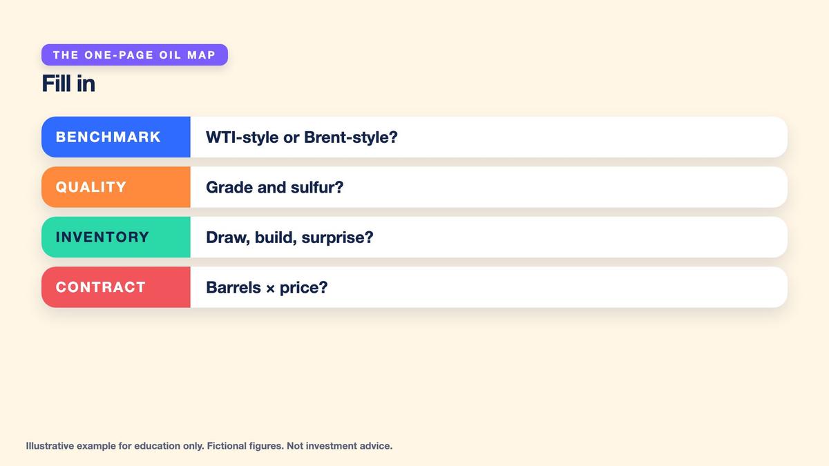
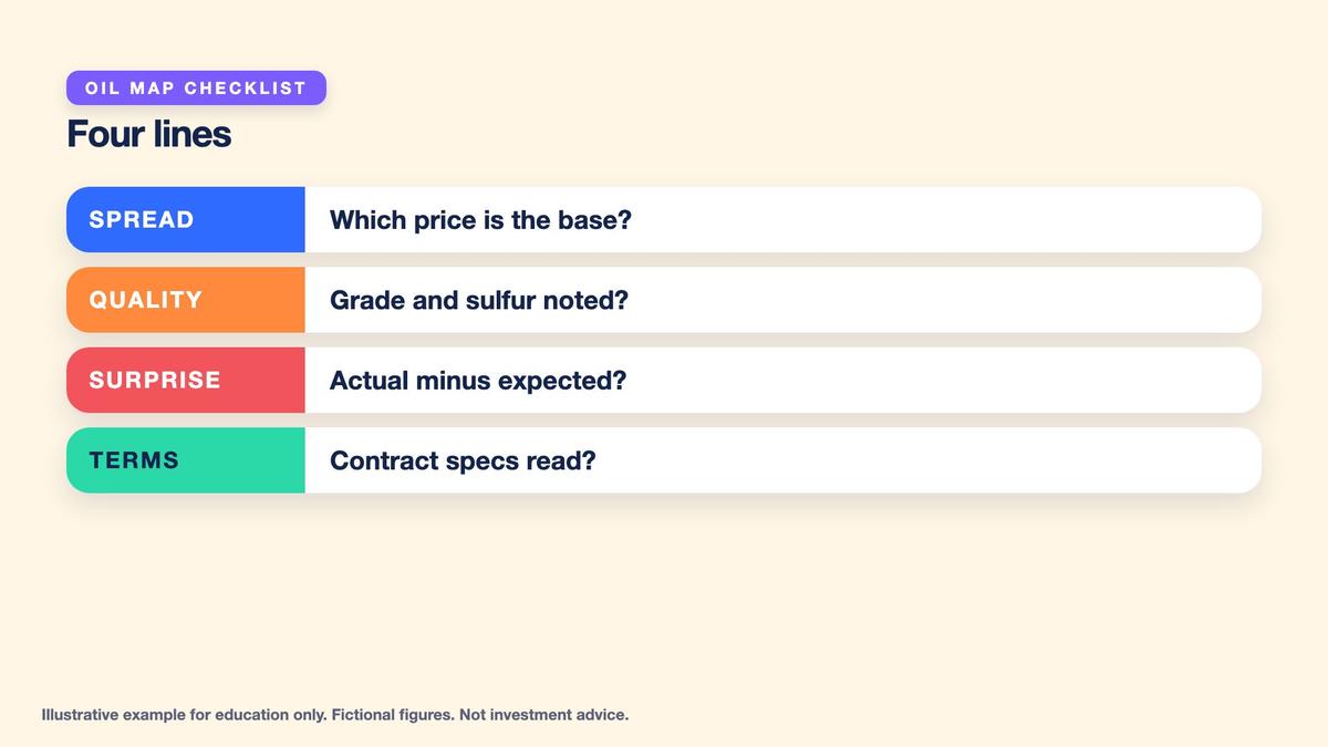
Begin the completed map with WTI and Brent as benchmark concepts rather than interchangeable commodities. Record the fictional WTI-style price of $70 and Brent-style price of $74, the $4 spread and the percentage denominators of 5.71% and 5.41%. Include the invented $2.50 transportation component and $1.50 quality-and-other component. Compare Sample Light Sweet at 40 degrees API and 0.4% sulfur with Sample Heavy Sour at 30 degrees API and 2.0% sulfur. Verify the fictional six-dollar heavy sour discount, $64 selling reference and approximately 8.57% discount relative to the $70 light sweet price.
Practice Lab: Build a Fictional Oil Benchmark and Inventory Map
Use only the invented WTI-style $70.00 and Brent-style $74.00 quotations, fictional crude quality samples, invented weekly inventory data, and fictional 1,000-barrel contract. Work step by step in a dated classroom research sheet. First calculate the four-dollar benchmark difference, both percentage denominators, the invented transport and quality decomposition, and the heavy sour grade discount. Next compare current crude stocks of 420.0 million barrels with the fictional 440.0 million five-year average, compute the weekly change from 422.5 million previously, compare actual change with the expected +1.0 million build, and interpret the surprise cautiously. Then calculate days of supply using 20.0 million barrels per day, hub utilization using 70.0 million capacity, and refinery throughput using 18.0 million barrels per day capacity. Finally convert the barrel prices into contract notionals and dollar movement sensitivity. All calculations are simulations, not actual published oil data or live trading.
- Decision 1: The fictional sample shows WTI-style oil at $70.00 per barrel and Brent-style oil at $74.00. The invented spread decomposition assigns $2.50 per barrel to transportation and $1.50 to quality and other factors. — Calculate the benchmark spread, the spread percentage using each benchmark denominator, and the invented transportation component across 1,000 barrels.
- Decision 2: Sample Light Sweet crude has 40 degrees API gravity and 0.4% sulfur. Sample Heavy Sour crude has 30 degrees API gravity and 2.0% sulfur, with a fictional six-dollar discount to the $70 light sweet reference. — Identify the lighter, lower-sulfur grade, calculate the heavy sour reference price and percentage discount, and explain why the discount is not universal.
- Decision 3: A fictional weekly report lists current crude stocks of 420.0 million barrels, previous stocks of 422.5 million, five-year average stocks of 440.0 million, and an expected weekly build of 1.0 million. — Calculate the actual weekly change, the surprise against expectations, the shortfall relative to the five-year average and its percentage, then interpret the result cautiously.
- Decision 4: Invented daily demand is 20.0 million barrels. A fictional storage hub has 70.0 million barrels of capacity and 21.0 million current stocks, with another scenario showing 56.0 million stocks. Refinery capacity is 18.0 million barrels per day. — Calculate days of supply, both storage utilization cases, and refinery crude processing at 90% and 95% utilization.
- Decision 5: The fictional oil contract represents 1,000 barrels, with benchmark quotations of $70 and $74 per barrel. The learner has not been provided actual margin, expiry or settlement specifications. — Calculate contract volume, dollar sensitivity, reference notionals and benchmark spread value, then identify what must be verified before any real-world contract comparison.
Answer key
Next reconcile the inventory section. Current crude stocks are 420.0 million barrels, below the invented five-year average of 440.0 million by 20.0 million or approximately 4.55%. Previous stocks were 422.5 million, giving an actual 2.5-million draw. An anticipated 1.0-million build means the actual-minus-expected surprise is negative 3.5 million. At fictional daily demand of 20.0 million barrels, inventory coverage is 21 days rather than 22 days at the historical average. Record the hub's 30% current utilization and 80% higher-inventory scenario, then verify refinery throughput of 16.2 million barrels per day at 90% utilization and 17.1 million at 95%.
Key points
- Fill in the oil map: benchmark and spread, quality, inventory surprise, days of supply, storage, refining and contract exposure.
- Reconcile: $4.00, 5.71%, -3.5M, 21 days, 80% and $70,000.
- Keep every signal as a clue, never a guarantee, and verify real contract terms.
Finish with the fictional 1,000-barrel contract, its 42,000-US-gallon volume, $1,000 profit-and-loss sensitivity per dollar of price movement, and reference notionals of $70,000 and $74,000. Add unanswered specification questions about margin, tick size, contract month, last trading day, delivery or cash settlement, trading hours and transaction fees. Journal any directional inventory interpretation as a conditional observation, not a forecast. This follows the earlier gold exposure map and XAUUSD sizing laboratory: normalize units, verify the instrument, calculate exposure, and document uncertainty before considering risk. All inputs are fictional, and no real trading decision is required.
Worked example at a glance
Key terms
- Barrel: a volume unit of 42 US gallons.
- Benchmark: a widely referenced price for a defined crude market.
- WTI: West Texas Intermediate, linked to inland North American crude.
- Brent: a benchmark linked to seaborne crude pricing.
- Spread: the price difference between two benchmarks.
- API gravity: a measure of how light or heavy a crude is.
- Sulfur: the sulfur content that separates sweet from sour crude.
- Inventory: crude held in storage at a point in time.
- Draw: a fall in inventories over a period.
- Build: a rise in inventories over a period.
- Days of supply: inventory divided by daily demand.
- Notional: barrels times price, the dollar size of a contract.
Multi Asset Trading Lab provides educational information only and does not constitute personalized investment, trading, commodities, futures, financial, accounting, tax, legal, energy-market, brokerage or risk-management advice. All oil prices, inventory statistics, crude quality measurements, benchmark spread components, expectations, demand assumptions, refinery figures, storage utilization levels, contract specifications, example prices and calculations in this lesson are fictional and created solely for classroom use. No real company, inventory report, oil dealer, financial instrument, exchange, broker, trading account, exchange contract code or current market price is used or recommended. The conventional meanings of WTI, Brent, API gravity, crude oil barrel volume, inventory builds and draws, and other broad market concepts are provided as educational definitions, not current market observations or product-specific trading instructions. WTI stands for West Texas Intermediate and is generally associated with inland North American crude oil pricing, while Brent is a major international crude benchmark associated with seaborne markets. Actual financial instruments referencing these benchmarks may have different grade definitions, delivery locations, settlement processes, contract multipliers, contract months, trading hours, margins and legal obligations. A real instrument's current official specifications must be independently verified before attempting to interpret its financial exposure. One standard oil barrel is 42 US gallons, approximately 159 liters. A barrel is a physical volume unit, not a fixed monetary value, a universal contract size or a guarantee of delivery rights. The fictional benchmark quotations of $70.00 per barrel for WTI-style crude and $74.00 for Brent-style crude are not actual or historical market quotations and must not be used in real investment decisions. Their four-dollar spread equals approximately 5.71% of the WTI-style reference or 5.41% of the Brent-style reference, depending on the denominator. The invented spread allocation of $2.50 per barrel for transportation and shipping plus $1.50 for quality and other factors is a teaching decomposition rather than an empirical explanation of a real spread. Benchmark spreads can be affected by crude quality, local supply, shipping, pipeline capacity, freight, inventories, demand, export access, contract specifications, timing, trading liquidity and other factors, and there is no universal fixed contribution from any one factor. The presence of a spread between benchmarks does not prove an executable, risk-free or profitable arbitrage opportunity. The fictional quality example compares Sample Light Sweet crude at 40 degrees API gravity and 0.4% sulfur with Sample Heavy Sour crude at 30 degrees API gravity and 2.0% sulfur. The invented six-dollar discount from a $70 reference yields $64 per barrel for the heavier, higher-sulfur sample and approximately an 8.57% relative discount. These fictional quality parameters and prices do not establish actual commercial grade specifications, typical discounts or future grade relationships. API gravity is related to density, with higher API values generally indicating lighter oil, while sulfur content is one of several characteristics affecting refinery processing. Crude value can also depend on refinery configuration, product yields, transportation, demand, processing costs and changing market conditions. No quality category alone guarantees a particular price or discount. The weekly crude inventory report in this lesson is entirely invented and is not an official statistical release. Its current stocks of 420.0 million barrels, previous stocks of 422.5 million barrels, five-year average of 440.0 million barrels and expected weekly build of 1.0 million barrels are hypothetical inputs. Current stocks are 20.0 million barrels below the invented historical average, corresponding to approximately 4.55% of that reference. Actual weekly inventory change is negative 2.5 million barrels, representing a draw. Actual change minus the expected positive 1.0 million build equals a negative 3.5-million-barrel surprise. A larger-than-expected draw may be interpreted as a potential signal of tighter conditions than anticipated, while a larger-than-expected build may signal looser conditions, but neither result guarantees that oil prices will move in a particular direction. Oil prices can already reflect expectations before publication and can respond to producer announcements, changes in production and demand, weather, refinery outages, import or export conditions, shipping disruptions, financial positioning, currency moves and other information occurring at the same time. A reported inventory change is not a direct observation of total global supply or demand and may depend on statistical coverage, timing, definitions or revisions. The classroom days-of-supply calculation divides fictional current inventories of 420.0 million barrels by invented demand of 20.0 million barrels per day, yielding 21.0 days. Applying the same fixed assumed demand to the 440.0-million five-year reference yields 22.0 days, one day more. These are simplified ratios and not literal predictions of when storage will empty, oil supplies will cease, or the economy will exhaust its resources. Production, imports, exports, consumption, refinery activity and inventory availability continuously change, and some stored barrels may not be commercially or operationally accessible. The fictional storage hub has 70.0 million barrels of nominal capacity and current stocks of 21.0 million barrels, giving 30% utilization. The hypothetical higher-inventory case uses 56.0 million barrels, giving 80% utilization. Nominal unused capacity is 49.0 million and 14.0 million barrels respectively. Actual operational capacity can differ from nominal design capacity because of tank maintenance, inventory segregation, minimum operating requirements, pipeline constraints, product quality, logistical scheduling and other restrictions. Higher storage fullness can pressure nearby physical deliveries in certain circumstances but does not establish any guaranteed price, price floor, threshold effect or future contract relationship. The fictional refinery system has daily processing capacity of 18.0 million barrels. At 90% utilization its calculated throughput is 16.2 million barrels per day, and at 95% utilization throughput rises to 17.1 million barrels per day, a difference of 0.9 million barrels per day. These are arithmetic scenarios rather than actual industry operating data. Crude refinery runs are not identical to total oil demand, final product consumption, storage withdrawals or refinery profit, and their economic interpretation depends on broader market conditions. The fictional contract used for price sensitivity represents 1,000 barrels, equivalent to 42,000 US gallons. At an invented $70 reference it has $70,000 notional exposure, and at an invented $74 reference it has $74,000. A $1.00 price movement per barrel creates $1,000 of gross contract value change in either direction under the stated linear assumption. The four-dollar difference between reference prices corresponds to $4,000 across 1,000 barrels, consisting of the classroom's invented $2,500 transport component and $1,500 quality-and-other component. These scaled calculations do not represent executable spread profits or the actual mechanics of simultaneously trading different benchmark instruments. Real oil financial contracts may differ in barrel quantity, tick size, tick value, denomination, exchange rules, margin, expiry, delivery obligations, settlement timing, price limits, physical storage requirements, roll procedures and liquidity. Notional value can be much larger than posted margin, and leverage can magnify losses relative to cash collateral. Physical delivery obligations, expiry and futures curve structures may introduce risks that are not present in this simplified introductory model. A trader may lose more than initially expected because of gaps, execution slippage, contract rollover, changes in spreads, liquidity shortages, broker or clearing requirements, margin calls, liquidation, fees or other conditions. The previous gold exposure map, XAUUSD contract sizing lab, spread and slippage material, and margin and leverage lessons provide conceptual frameworks but do not make trading safe or outcomes predictable. The figures in this lesson do not establish an appropriate contract size, risk budget, stop level, trading direction, holding period or strategy. The required exercise is a one-page simulated oil market map that records assumptions, benchmark definitions, quality characteristics, inventory calculations, storage and refinery measures, contract sensitivity and unanswered specification questions. Its goal is to improve understanding of physical oil pricing and inventory interpretation, not to forecast prices or generate a trading signal. All exercises use simulated money and fictional inputs only. Nothing in this lesson recommends buying, selling, holding, hedging, borrowing against, or trading any actual commodity, security, future, option, CFD or other financial instrument. No real-money trading, account opening, physical delivery or financial commitment is required or encouraged.
Lesson Checkpoint
Review what you learned and get feedback on your work.